Flying a quadcopter in Simulink with cascaded PID

QuadX is a quadcopter modelled from first principles in MATLAB/Simulink and stabilised with cascaded PID control. It was a five-person project for EE291 System Dynamics and Control at Maynooth. I worked on the mathematical modelling, the PID design and tuning, and the Simulink implementation, and acted as the team’s main contact with our facilitator.

It’s simulation only: no physical drone was built. The model, parameters and reports are on GitHub.

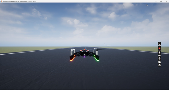
The vehicle

Parameter	Value
Mass	1.5 kg
Arm length	0.25 m
Inertia	Ix = Iy = 0.02, Iz = 0.04 kg·m²
Thrust per rotor	0–15 N, saturated

Ix equals Iy because the cross frame is symmetric. Iz is double because all four rotor masses sit at full arm length from the yaw axis. Hover needs m·g = 14.72 N in total, or 3.68 N per rotor: about a quarter of each rotor’s ceiling, which leaves room for attitude corrections.

Dynamics

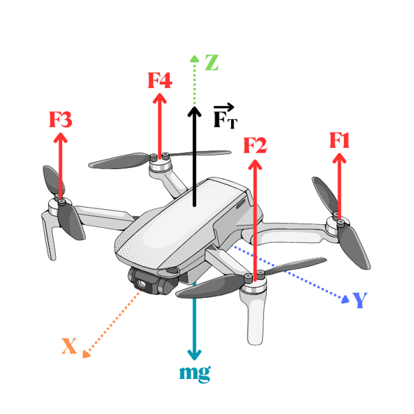
Translation and rotation are derived separately from free-body diagrams and built as separate Simulink subsystems, one per axis, each integrating acceleration to velocity to position.

• Translation is Newton’s second law in the inertial frame. Total thrust acts along the body z-axis. Tilting the body projects part of that thrust sideways, which is the only way a quadcopter moves horizontally. Gravity is the only other force.
• Rotation is Euler’s equations in the body frame. Roll comes from a thrust difference between the left and right rotors, pitch from front and rear, and yaw from the reaction drag between the clockwise and counter-clockwise pairs.

Four setpoints, six degrees of freedom

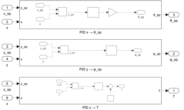
The controller only ever receives four setpoints: x, y, z and yaw. Roll and pitch are never commanded directly. That works because the controller has two nested loops.

The outer loop handles position. It turns horizontal position error into a desired acceleration. Since horizontal acceleration comes from tilting thrust, the required tilt follows from dividing by g and taking the arcsine. Those angles become roll and pitch setpoints.

The inner loop handles attitude. It tracks the roll, pitch and yaw setpoints by commanding a torque about each body axis.

A mixing matrix converts the four controller outputs (total thrust plus three torques) into individual rotor thrusts:

[ 1   1   1   1 ]   thrust
[ 1  -1  -1   1 ]   roll torque
[ 1  -1   1  -1 ]   pitch torque
[ 1   1  -1  -1 ]   yaw torque

Each rotor’s output is then clamped to 0–15 N, so the simulation respects actuator limits. That matters, because saturation is exactly where cascaded PID tends to misbehave under large setpoint steps.

Tuning

The full dynamics are nonlinear and strongly coupled, so classical PID design has nothing to work with directly. We linearised the model about hover with Simulink’s linear analysis tools, which gave transfer functions for step response and root locus work. Simulation then refined the gains.

Loop	P	I	D
Roll, pitch, yaw	1.18	0.6	0.3
Position x	1.4	0.4	2.2
Position y	1.2	0.5	1.4
Altitude z	2.5	0.6	0.85

The pattern in the gains is the interesting part. On x and y, derivative gain is larger than proportional gain. Horizontal corrections have to travel through the attitude loop before they move the vehicle, which adds phase lag, and the D term damps it. Altitude is the opposite: z acts directly on total thrust with no inner loop in between, so proportional gain does most of the work.

Validating bottom-up

We tested each subsystem on its own before connecting anything: motor mixing, motor model, translational dynamics, rotational dynamics. When the closed loop later misbehaved, we already knew the plant was right, so the fault had to be in the controller. That saved a lot of guessing.

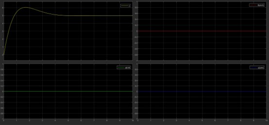
The final tests were a hover hold and an approach to x = 0, y = 0, z = 5 m with zero yaw.

What I’d change

• Yaw shares roll and pitch’s gains despite having double the inertia, so it has roughly half the effective authority. It works, but it was inherited rather than tuned.
• The controller reads perfect state straight from the simulation. A real vehicle would need a state estimator, such as a Kalman filter fusing IMU data, and we never built one.
• No drag, wind or motor lag. Any of them would degrade the tuned gains.
• No benchmark. LQR is the natural comparison for a coupled multi-input system like this. Without it, there’s no evidence PID was the best choice rather than the familiar one.

The parameters and gains are in model/init_params.m if you want to run it yourself.